Object segmentation using deep neural networks
Deep neural networks are supervised machine learning methods amenable for application to complex, non-linear classification tasks. For this reason, training is significantly more computationally expensive than in the case of linear classifiers. PyJAMAS implements U-Net, a deep neural network architecture.
The training dataset consists of a set of images of the structure to be detected (cells, nuclei, etc.) and corresponding binary image masks labelling the objects in the input images. During training, a loss function measures how far the network prediction is from the target segmentation. The loss function is weighed with a map that has greater values at pixels in the proximity of the edges of structures. Increasing the weight of edge pixels penalizes segmentation errors at boundaries and ensures that the network learns to separate structures in close contact.
Creating training sets
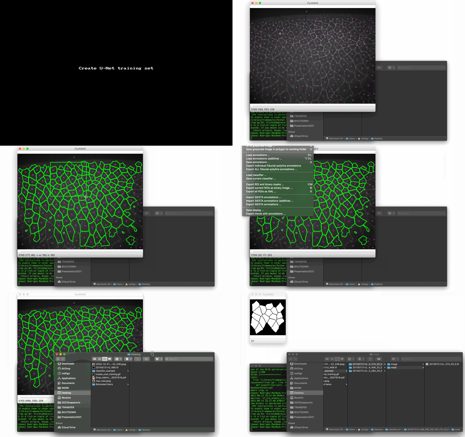
Open a grayscale image or time-lapse sequence that includes examples of the structure to be detected (e.g. cell nuclei).
Set the working folder using Set working folder … under the Options menu. Training images will be automatically saved into the working folder.
Outline the structures to be detected by the classifier. This can be done using any of the tools (rectangles, polylines, LiveWires) available in PyJAMAS, in the entire image or in subregions thereof.
Draw a rectangle (ROI) around a small group of segmented structures.
Save the region of the image within the rectangle and a binary mask corresponding to the outlined structures using Export ROI and binary masks … from the IO menu. You will need to click on the rectangle ROI. A subfolder will be created inside the working folder. The subfolder name is a combination of the name of the original image, the XY coordinates of the subimage, and the slice number. The new subfolder in turn contains two subfolders, one with the ROI image and one with the binary mask.
Move the rectangle ROI to a different location using the Move polyline option from the Annotations menu. Click and drag the rectangle to the desired position. The cursors can be used to further refine the position of the rectangle.
Repeat the steps above until you have a collection of images of the structure to be segmented. These images constitute the training set. Make sure that your training set represents the diversity of shapes and intensities of the structure to be detected. In general, the more examples, the better. We typically use 100-300 images in our training sets, but we have obtained classification accuracies greater than 90% using 80 images.
Training a U-Net
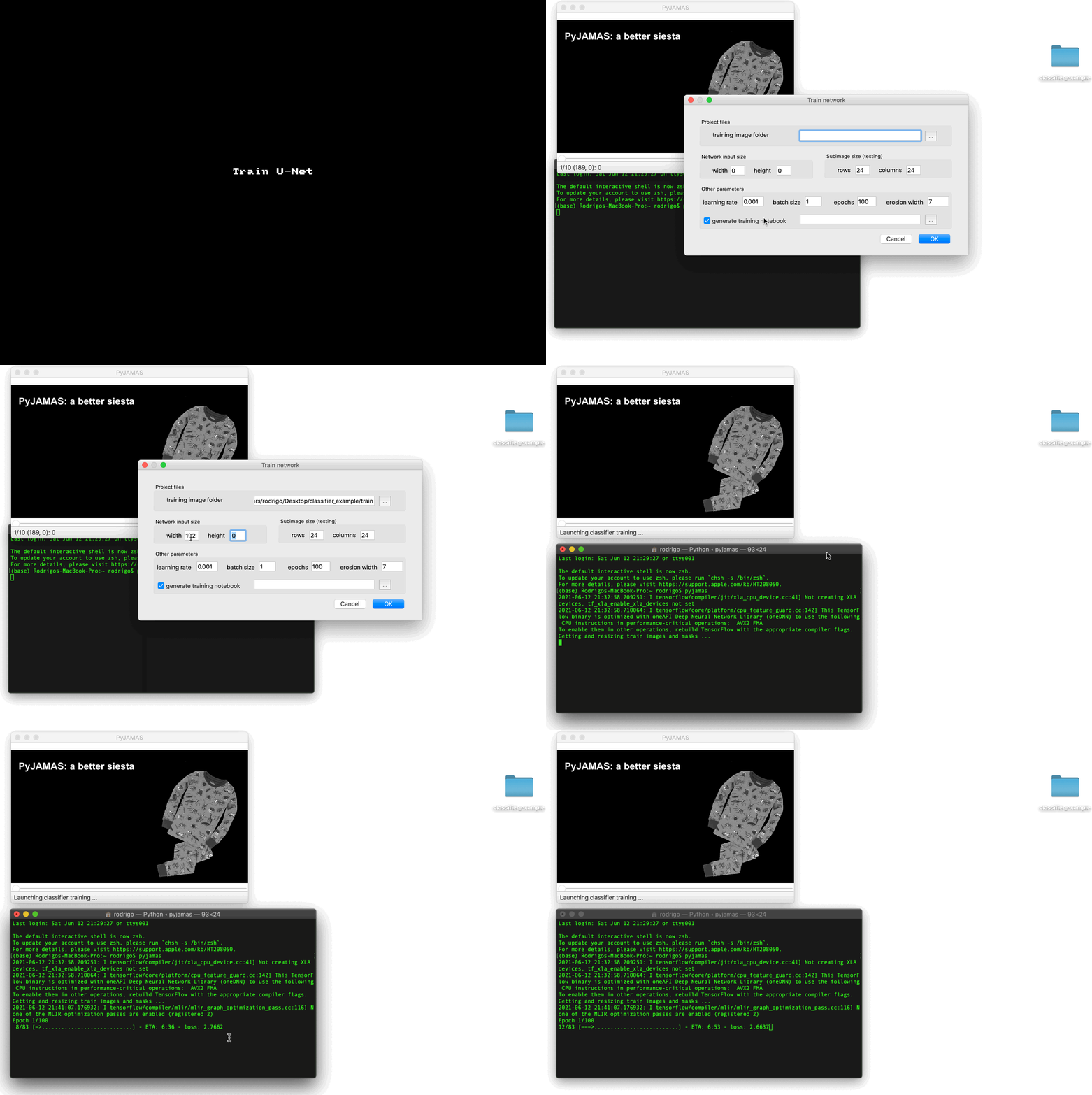
Select Create and train UNet … from the Image, Classifiers menu.
Fill in the parameter values to train the U-Net:
training image folder: path to the folder containing the training set.
network input size: the width and height of the images that will be fed into the network. Training images will be rescaled to this size. Because of the architecture of the network, the selected dimensions must be divisible by 16 (but not necessarily equal to each other). Smaller input images generate smaller networks with fewer parameters that train faster. However, smaller networks are worse at resolving boundaries between touching structures. 32x32, 64x64, 128x128 or 192x192 are typical values.
subimage size (testing): number of pixel rows and columns to divide test images into (post training, when the networks is applied to new images). Each subimage will be scaled to the network input size and processed. Decreasing the subimage size leads to increased object detection resolution, at the expense of longer processing times. Increasing the step size accelerates image classification but can reduce its accuracy.
learning rate: scale factor that affects the step size when minimizing the cost function of the network. Larger values lead to faster training, with the possibility of missing cost function minima. Smaller values are more likely to converge to the minimum of the cost function, but take longer to get there.
batch size: number of images in the training set that are propagated through the network before updating the weights. Smaller values result in a noisy minimization of the cost function and slower learning, but the trained networks are more generalizable. A typical value is 32.
epochs: number of times that the entire training data set will be run through the network.
erosion width: size of the erosion kernel applied to the binary image produced by the trained network when applied to a new image.
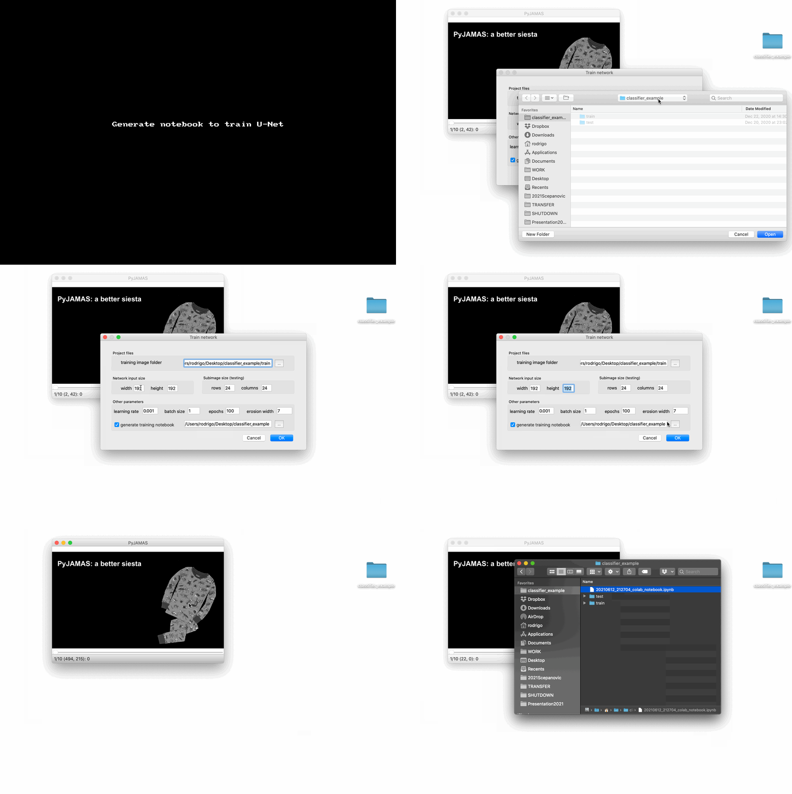
generate training notebook: training a neural network is computationally expensive. If you are not running the training in a computer equipped with a Graphics Processing Unit (GPU), it may take a long time for training to finish. Thus, PyJAMAS offers the possibility of generating a notebook that can be uploaded together with the training data to platforms such as Colab for faster training. Colab offers free remote access to GPU-equipped machines. When executed on Colab, the notebook generated by PyJAMAS will train the network and save a model that can be used in Colab or downloaded and loaded into PyJAMAS for application to new images. Check this box to generate the notebook (saved at the path indicated on the textbox to the right) and train remotely, or leave unchecked to run the training on the local computer.
Select OK and wait for the network to be trained. A message on the status bar will indicate training completion.
Save the trained network using the Save current classifier … option from the IO menu. Or run the notebook in Colab and download the trained networks.
Trained networks can be loaded using the Load classifier … option from the IO menu.
Training a U-Net in Colab
When you create the U-Net, make sure to check generate training notebook.
In the selected folder, a new file with .ipynb extension (a notebook) will be created.
Upload the notebook and both train and test data to Colab. Make sure that your connection is to a runtime equipped with a GPU (you can validate this with the Change runtime option under the Runtime menu). The notebook assumes that both train and test data will be uploaded in a zip file named testtrain.zip. But this is easy to edit in the notebook. It is important to store each training image in an independent folder, each of which contains two subfolders, image and mask, that in turn contain the training image and the binary mask highlighting the objects, respectively.
In Colab, run through the notebook. Training will take some time. When training is done, make sure to download the generated model.
Using a U-Net
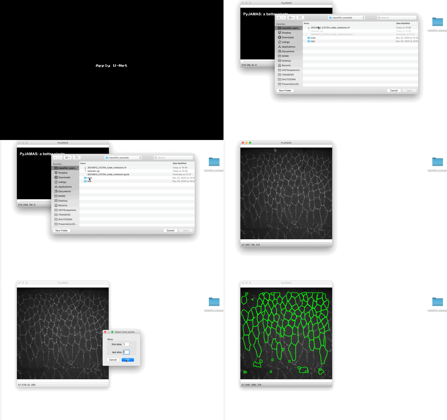
To detect structures in an image using a U-Net, open the image and make sure to train a network or load a trained network.
Select Apply classifier … from the Image, Classifiers menu, and choose the slices to apply the network to.
PyJAMAS will add a polyline annotation around each of the objects detected by the classifier.
