Object segmentation using QuickieNets
A QuickieNet is a ReSCU-Net that rather than attempting to individually segment and track each one of the objects in an image, segments and tracks all the existing objects simultaneously. “Existing” is determined by the presence of the object in the user-provided prompt that annotates “all” the objects of interest on the previous image in the sequence.
To segment objects in an image, QuickieNets use the image data, as well as the segmentation mask of the objects from the previous timepoint.
The training dataset consists of a set of images of the objects to be detected (cells, nuclei, etc.), corresponding binary image masks labelling the objects in the input images, and binary image masks labelling the same objects in the previous timepoint. During training, a loss function measures how far the network prediction is from the target segmentation. The loss function is weighed with a map that has greater values at pixels in the proximity of the edges of structures. Increasing the weight of edge pixels penalizes segmentation errors at boundaries, ensuring that the network can correctly find object boundaries.
Because a QuickieNet does not learn “individual” objects, it is significantly faster than the corresponding ReSCU-Net, and requires less pre-processing of the training images. But speed comes with some tradeoffs:
QuickieNets assume that the same number of objects is present in all images.
QuickieNets require at least some overlap between corresponding objects in consecutive images in the sequence.
QuickieNets may be somewhat less accurate than ReSCU-Nets.
Creating training sets
Outline the objects to be detected by the classifier. This can be done using any of the tools (rectangles, polylines, LiveWires) available in PyJAMAS, in the entire image or in subregions thereof. When outlining objects, ensure that each object is drawn in the same order on each frame so that the object ids are unchanged throughout timepoints. (Object ids can be shown by toggling Display fiducial and polyline ids in the Options menu, and you can edit polyline ids with this PyJAMAS ids_plugin).
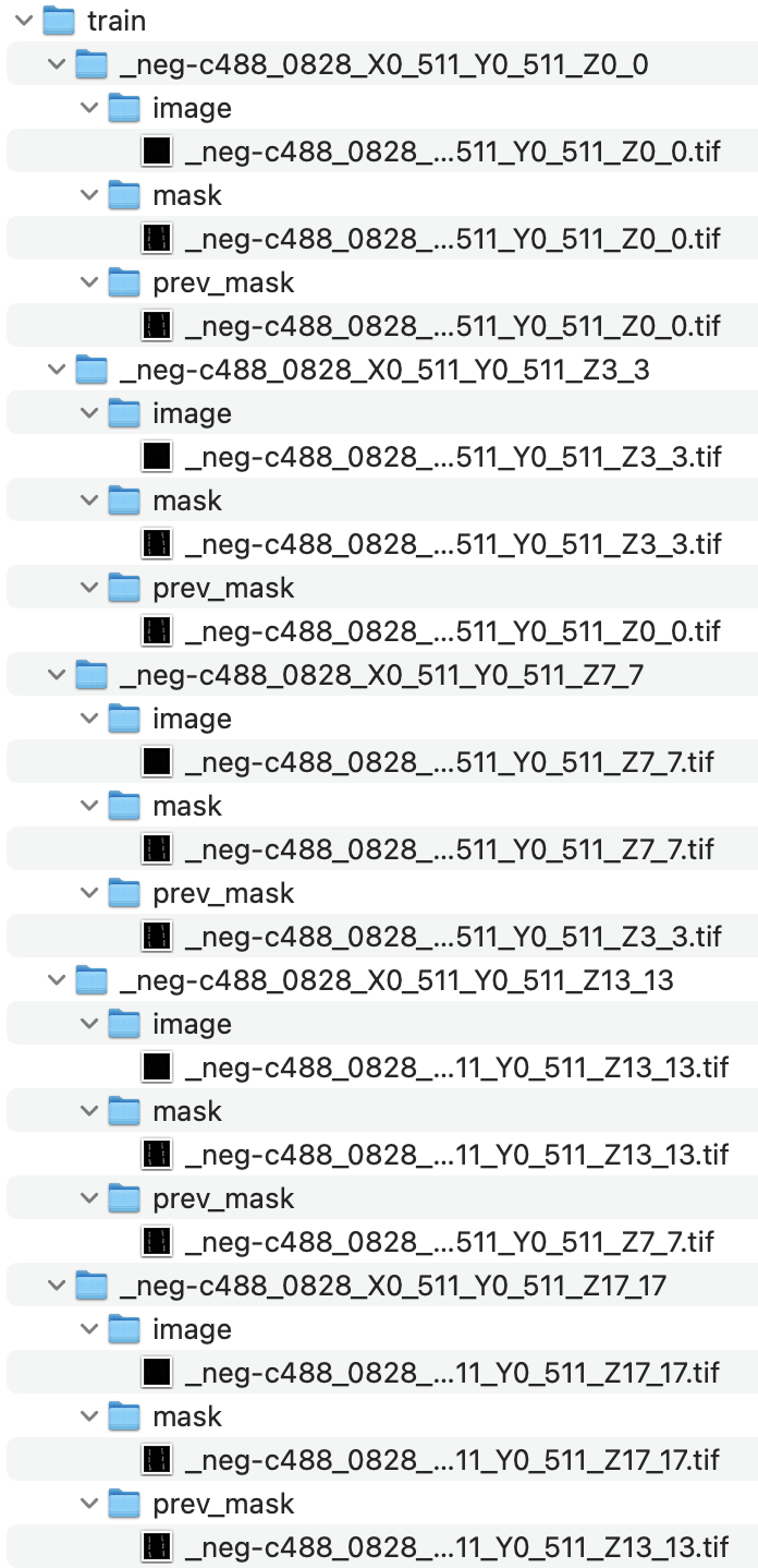
Using your segmentations create a training dataset in a parent folder where each subfolder corresponds to a specific object at a specific timepoint. Each subfolder should have folders for the image at the current timepoint, object mask for the current timepoint, and object mask for the previous timepoint.
This PyJAMAS training_plugin automatically generates a training dataset from a set of movies and PyJAMAS annotation files (.pjs).
Training a QuickieNet
Select Create and train QuickieNet … from the Image, Classifiers menu.
Fill in the parameter values to train the QuickieNet:
training image folder: path to the folder containing the training set.
save folder: path to the folder where model checkpoints, training logs and the final model will be saved.
generate training notebook: training a neural network is computationally expensive. Training in a computer without a Graphics Processing Unit (GPU) may take a long time. Thus, PyJAMAS offers the possibility of generating a notebook that can be uploaded together with the training data to platforms such as Colab for faster training. Colab offers free remote access to GPU-equipped machines. When executed on Colab, the notebook generated by PyJAMAS will train the network and save a model that can be used in Colab or downloaded to be used locally through PyJAMAS. Check this box to generate the notebook (saved at the folder indicated on the textbox to the right) and train remotely, or leave unchecked to run the training locally.
network input size: the width and height of the images that will be fed into the network. Because of the architecture of the network, the selected dimensions must be divisible by 16 (but not necessarily equal to each other). Smaller input images generate networks that train faster. However, smaller networks are worse at resolving boundaries between touching structures. Training images will be rescaled to this size. If the network image size is much smaller than the training images, it is recommended to generate training images that are cropped to the network input size so that resolution is not lost during down sampling. 32x32, 64x64, 128x128 or 192x192 are typical values.
step size (testing): when applying the network to new images that are larger than the network input size, the image will be tiled into subimages. Subimages will be taken every step size pixels across the image. Increasing the step size accelerates image classification but can reduce accuracy. NOTE: this value can be changed after training, using the Image > Classifiers > Change neural net step size … option. A recommended value is the network input size divided by 2, which leads to 50% overlap between subimages.
learning rate: scale factor that affects the magnitude of weight updates when minimizing the cost function of the network during training. Larger values lead to faster training, with the possibility of missing cost function minima. Smaller values are more likely to converge to the minimum of the cost function, but take longer to get there.
batch size: number of images in the training set that are propagated through the network before updating the weights. Smaller values can result in a noisy minimization of the cost function, slower learning, and overfitting. Larger values can exceed the available memory or result in underfitting. A typical value is 32, but can be reduced down to 1 for large images.
epochs: number of times that the entire training data set will be run through the network.
validation split: fraction of training images to set aside for validation. At the end of each training epoch the network will be applied to the validation images and a validation loss will be measured, allowing the training protocol to measure and prevent overfitting.
erosion width: size of the erosion kernel applied to the binary image produced by the trained network when applied to a new image.
concatenation level: the number of encoder blocks that the image and previous mask are processed separately before being combined. A concatenation level of 1 works well for most datasets, but higher concatenation levels can improve accuracy if objects change a lot between timepoints (max. 4). Increasing concatenation level increases the size of the network, leading to longer training and prediction times.
early stopping: if checked, the training protocol will monitor the validation loss and stop training early if the validation loss does not improve after patience epochs. If training is stopped early, the epoch with the best validation loss will be saved at the end of training. Do not use this function if your validation split is 0.0. Use this function with save model checkpoints to ensure that the best model is saved even if training is not stopped early.
learning rate scheduler: if checked, the training protocol will monitor the validation loss and reduce the learning rate by a factor of 10 if the validation loss does not improve after patience epochs. Enabling this functionality leads to more stable training.
save model checkpoints: if checked, the model will be saved at the end of each epoch and at the end of training. If save best weights only is checked, the model will be saved to the save folder only if performance has improved, overwriting the previous best model. At the end of training, the best weights will be reloaded before the final checkpoint is saved. If save best weights only is not checked, the model will be saved at the end of each epoch to separate files (not recommended due to increased computation time and storage space).
logging: if checked, training and validation loss will be logged to TensorBoard at the end of each epoch. TensorBoard allows you to to generate training and validation loss plots as training is progressing. TensorBoard can be launched from the command line using “tensorboard –logdir /path/to/logs”, generating a link to visualize training progress in your browser.
Select OK and wait for the network to be trained. A message on the status bar will indicate training completion.
Save the trained network using the Save current classifier … option from the IO menu. Or run the notebook in Colab and download the trained networks.
Trained networks can be loaded using the Load classifier … option from the IO menu.
Training a QuickieNet in Colab
When you create the QuickieNet, make sure to check generate training notebook.
In the selected folder, a new file with .ipynb extension (a notebook) will be created.
Upload the notebook and both train and test data to Colab. Alternatively, upload the train and test data to your google drive, open the training notebook in Colab, and mount your google drive. Edit the path in which training data are saved. It is important to store each training image in an independent folder, each of which contains three subfolders: image, mask, and prev_mask, that in turn contain the current image frame, the binary mask highlighting the object in the current frame, and the binary mask highlighting the object in the previous frame, respectively.
Make sure that your connection is to a runtime equipped with a GPU (you can validate this with the Change runtime option under the Runtime menu).
In Colab, run through the notebook. Training will take some time. When training is done, make sure to download the generated model.
Using a QuickieNet
To detect structures in an image using a QuickieNet, open the image and make sure to train a network or load a trained network.
Outline the objects in the first slice that you wish to segment.
Move to the next or previous slice (QuickieNets can work forward or backwards!).
Option 1: segment entire videos at once (works well if you have few objects on each frame, or a network with very high accuracy)
Select Apply classifier … from the Image, Classifiers menu, and choose the slices to apply the network to. If you want to apply the QuickieNet backwards, select first the frame with the greatest index.
PyJAMAS will add a polyline annotation around each of the objects detected by the classifier.
If the network performs poorly on some slices, you can correct the erroneous segmentation for the first incorrect slice, then reapply the network for the following slices.
Option 2: segment videos frame-by-frame (works well if you have many objects, or objects that are difficult for the network to segment)
Select Apply classifier to current slice … from the Image, Classifiers menu (or use the Shift+A shortcut).
Correct any erroneous segmentations produced by the network.
Advance to the next slice (or go back to the previous slice) and repeat.